[Toc]
An Auto-Encoder (AE) is mapping that encodes the input data into a lower dimensional representation that contains sufficient information to reconstruct the original input. An autoencoder incorporates two elements:
- An encoder that compresses the data into (encoding)
- A decoder that reconstructs the input given the encoding
We'll use the following notations:
- $$x \in \rm{I!}{R}^d$$ an input instance
- $z \in \rm{I!}{R}^k$ an encoding instance
- $f:x \in \rm{I!}{R}^d \mapsto z = f(x) \in \rm{I!}{R}^k$ the encoder
- $g:z\in \rm{I!}{R}^k \mapsto x = f(x) \in \rm{I!}{R}^p$ the decoder
Example
Let's use a neural network $f_\theta$ for our encoder and another network $g_\psi$ for the decoder on the MNIST dataset. We create our Python environment and install PyTorch:
python3 -m venv vae
source vae/bin/activate
# using CPU
# WHEEL_SOURCE="https://download.pytorch.org/whl/cpu"
# using CUDA
WHEEL_SOURCE="https://download.pytorch.org/whl/cu118"
pip3 install torch torchvision torchaudio --index-url $WHEEL_SOURCE
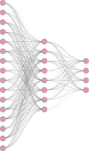
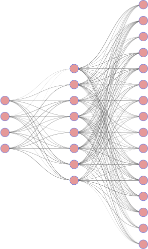
The MNIST dataset are 28x28 (d=784 pixels) grayscale images of digits. We define a simple encoder/decoder where the code has dimension k=32.
 |
 |
|---|---|
| encoder | decoder |
import torch
from torch import nn

device = torch.device('cpu')
if torch.cuda.is_available():
    device = torch.device("cuda")

d = 784
k = 16
encoder = nn.Sequential(nn.Linear(d, 256),
                        nn.LeakyReLU(),
                        nn.Linear(256, k),
                        ).to(device)

# note that the input is in [0,1], so we use the Sigmoid activation to map the
# reconstruction to [0,1]
decoder = nn.Sequential(nn.Linear(k, 256),
                        nn.LeakyReLU(),
                        nn.Linear(256, d),
                        nn.Sigmoid()
                        ).to(device)
# Optimizer to use for gradient descent
optimizer = torch.optim.Adam(params=
                             list(encoder.parameters()) + list(
                                 decoder.parameters()),
                             lr=1e-3)
The simplest reconstruction loss is perhaps the Mean Squared Error (MSE). The reconstruction loss for a single sample $x$:
$$ L_{\theta, \psi}(x) = ||x -f_\theta\circ g_\psi (x)||^2 $$
For multiple samples, we average the samples' reconstruction losses.
loss_fn = nn.MSELoss()
Let's load our dataset and create the data loader for the training phase:
from torchvision.datasets import MNIST
from torch.utils.data import DataLoader
from tqdm import tqdm

mnist = MNIST(root="./data/MNIST", train=True, download=True)
print(mnist.data.shape)
# > (60000,28,28)
# scale images from [0,255] to [0., 1.]
mnist.data = mnist.data / 255.
# we reshape the data to match the expected input
dataloader = DataLoader(mnist.data.view(-1, d),
                        batch_size=32,
                        shuffle=True, num_workers=2)
We train for 5 epochs:
from tqdm import tqdm

num_epochs = 5
for e in range(num_epochs):
    epoch_loss = 0.0
    for batch in tqdm(dataloader):
        batch = batch.to(device)
        loss = loss_fn(batch, decoder(encoder(batch)))
        optimizer.zero_grad()
        loss.backward()
        optimizer.step()
        epoch_loss += loss.detach().cpu().numpy()
    print(f"Epoch {e} loss {epoch_loss / len(dataloader):.3f}")

# > Epoch 0 loss 0.024
# > Epoch 1 loss 0.014
# > Epoch 2 loss 0.012
# > Epoch 3 loss 0.011
# > Epoch 4 loss 0.011
Let's now examine some reconstructed examples:
- Reconstruct same random samples:
choice = [100, 14234, 6906, 300, 349]

original = mnist.data[choice]
# in inference-only, no need to store the backward graph
with torch.no_grad():
    # we have to pay attention to the input dimensions
    reconstructed = decoder(encoder(original.view(-1, d).to(device)))
    # transform the flattened reconstruction back to square image
    reconstructed = reconstructed.view(-1, 28, 28).cpu()
- Plot the examples:
import matplotlib.pyplot as plt
fig, ax = plt.subplots(2, len(choice))
for i, pair in enumerate(zip(original, reconstructed)):
    for j in range(2):
        ax[j, i].axis('off')
        ax[j, i].imshow(pair[j])
plt.subplots_adjust(wspace=0.1, hspace=0.1)
# save the output to file if needed
# plt.savefig("reconstruct.png", transparent=True)
plt.show()
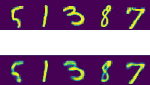
Original samples in row 1, reconstructions in row 2
And this is the easiest way to implement a simple Auto-Encoder to encode the 784 pixel into a representation of 16 dimensions.
Exploiting the encoded data
We can use the encoding instead of the original data in many other downstream tasks (classification, clustering, generative models). Let's see how the TSNE embedding of the code matches with the true images labels.
- First, we take a random subset of our data since the TSNE computes the pairwise distances and can be expensive to run on $60000^2$:
import numpy as np
# subset of size 2000
subset = np.random.choice(len(mnist.data), 2000, replace=False)
x = mnist.data[subset].view(-1, d)
y = mnist.targets[subset]
with torch.no_grad():
    code = encoder(x.to(device)).cpu()
- Embed the codes using a 2-components TSNE:
from sklearn.manifold import TSNE

embeddings = TSNE(n_components=2).fit_transform(code)
- Scatter plot the subset:
plt.set_cmap("rainbow")
plt.axis("off")
for yy in range(10):
    idx = (y == yy)
    plt.scatter(embeddings[idx, 0], embeddings[idx, 1], s=2, label=yy)

plt.legend(bbox_to_anchor=(0.0, 0.75), markerscale=2)
# save the plot if needed
# plt.savefig("tsne.png", transparent=True)
plt.show()
Scatter plot of 2d TSNE embedding of the encodings colored based on digit labels
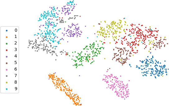
It looks good for an unsupervised learning (we did not have to use the true labels in the training)!